Discrimination
- Separating objects in an existing data set
- Find which variables that best separate the \(g\) groups
Classification
- Predict group membership for a new observation
- Allocate new objects to known groups
2018
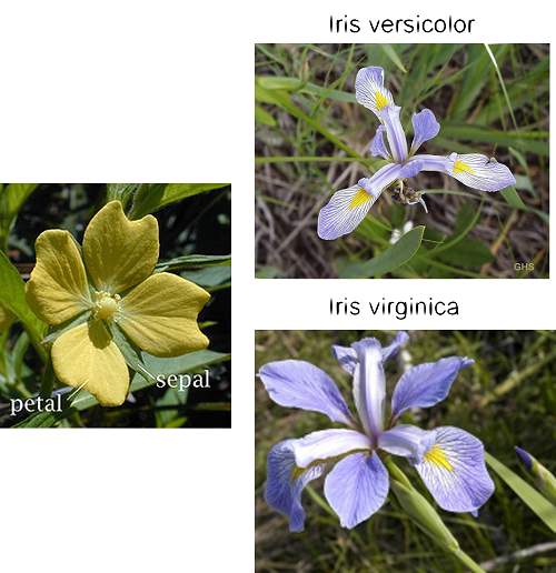
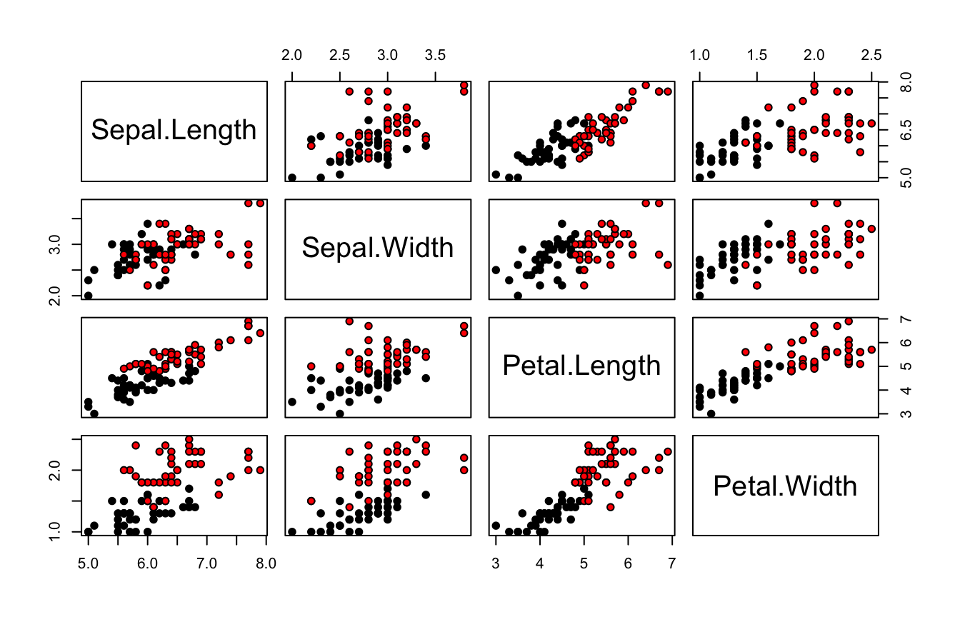
This famous (Fisher’s or Anderson’s) iris data set gives the measurements in centimeters of the variables:
X1)X2)X3)X4)load("_data/iris.train.Rdata")
head(iris.train)
   Sepal.Length Sepal.Width Petal.Length Petal.Width    Species
61          5.0         2.0          3.5         1.0 versicolor
62          5.9         3.0          4.2         1.5 versicolor
63          6.0         2.2          4.0         1.0 versicolor
64          6.1         2.9          4.7         1.4 versicolor
65          5.6         2.9          3.6         1.3 versicolor
66          6.7         3.1          4.4         1.4 versicolor
pairs(iris.train[, -5], bg = iris.train[, "Species"], pch = 21)
load("_data/Lizard.Rdata")
pairs(Lizard[, -4], bg = Lizard$Sex,
      pch = 21, cex = 1.5)
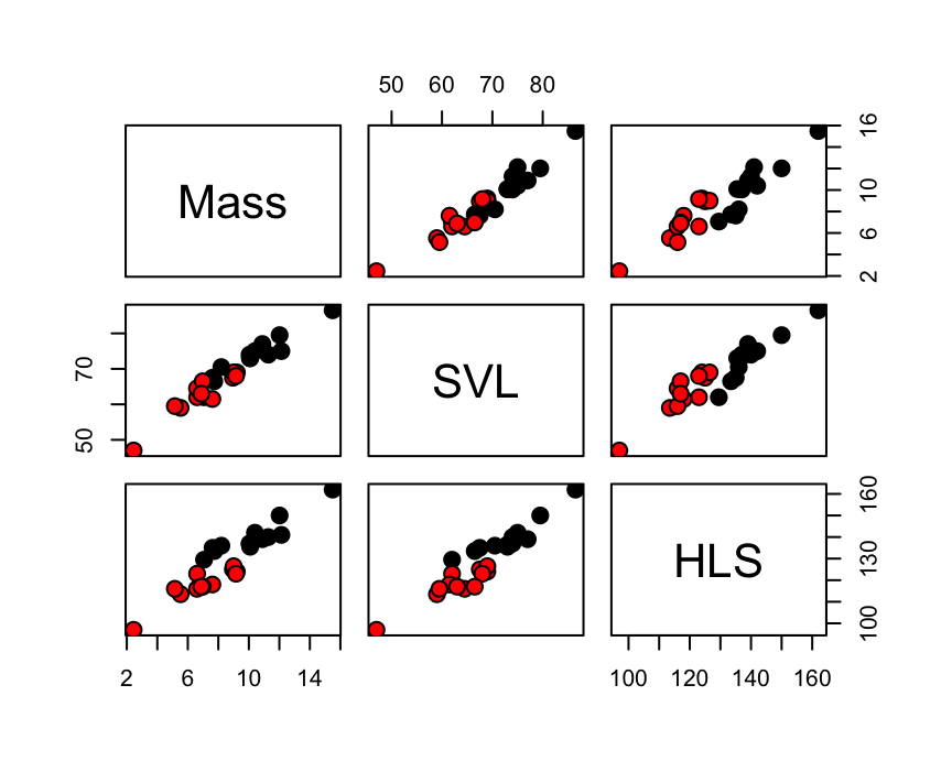
| variable | Description |
|---|---|
Mass
|
Weight of Lizard (in grams) |
SVL
|
Snout-vent length (in mm) |
HLS
|
Hind limb span (in mm) |
You must enable Javascript to view this page properly.
head(Lizard)
    Mass  SVL   HLS Sex
1  5.526 59.0 113.5   f
2 10.401 75.0 142.0   m
3  9.213 69.0 124.0   f
4  8.953 67.5 125.0   f
5  7.063 62.0 129.5   m
6  6.610 62.0 123.0   f
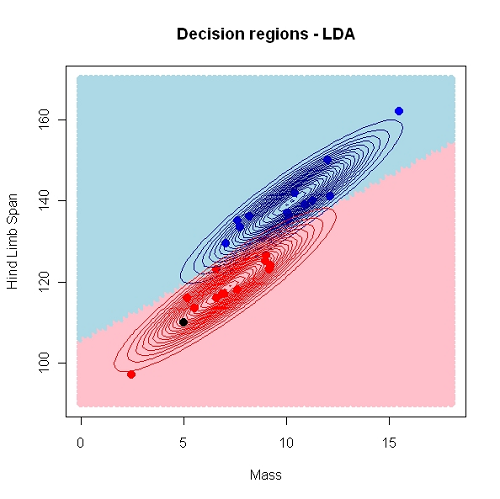
In descriminant analysis we search for decision regions for the \(g\) known groups (classes).
Regions \(R_1, R_2, \ldots, R_g\)
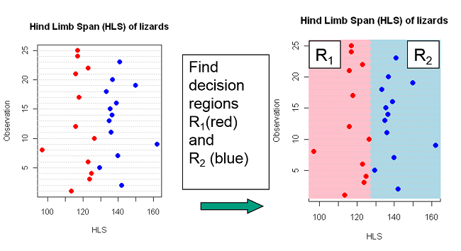
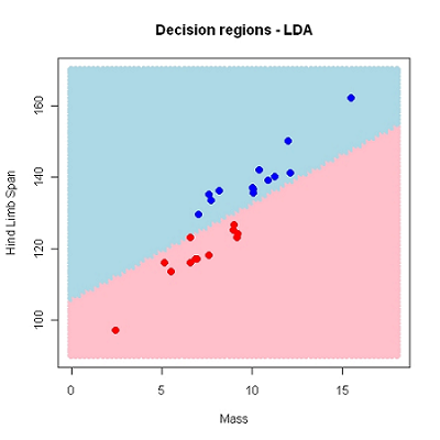
Using HLS and Mass as predictors \((k=2)\), we have used a linear decision border. This may also be non-linear.
You must enable Javascript to view this page properly.
Perfect discrimination/classification may not be possible.
The idea is to find decision regions \(R_1, R_2, \ldots, R_g\) that minimizes the probability of doing misclassification.
Intuitively we would allocate an observation to the group which is most probable given the observed value of the predictors
If, for example, the HLS of a new lizard is 130, it seems most probable based on previous data that the lizard is a male.
Let \(P(c_i|x_1,\ldots, x_p)\) be the probability of class \(i\) given the observed variables.
Then by Bayes rule:
\[P(c_i|x_1,\ldots, x_p) \propto f(x_1,\ldots, x_p|c_i)p_i\]
where \(p_i\) is the a priori probability of observing an object from class \(c_i\) and…
\(f(x_1,\ldots, x_p|c_i)\) is the likelihood (“probability”) of the observed data given class \(i\).
Allocate a new observation with observed variables \(x_1^*, x_2^*, \ldots x_p^*\) to the class which maximizes
\[f(x_1^*,\ldots, x_p^*)p_i\]
We need to estimate \(f(x_1^*,\ldots, x_p^*)\) from the training data and determine \(p_i\).
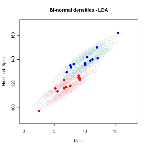
In linear discriminant analysis (LDA) we assume that \(f(x_1^*,\ldots, x_p^*)\) is a normal distribution, hence we must estimate the mean and (a common) variance for observations from each class.
Often we assume uniform prior: \(p_1 = p_2 = \cdots = p_g = 1/g\) .
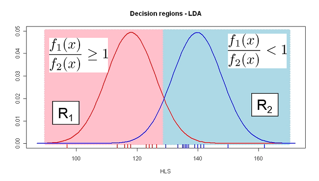
Assume equal probabilities for females (\(c_1\)) and males (\(c_2\)) a priori: \(p_1 = p_2 = 0.5\)
Assume \(x_1\) = HLS is the only predictor.
From the data we estimate \(\mu_1\), \(\mu_2\) and common \(\sigma^2\) for both classes. Let \(f_1\) and \(f_2\) denote these two normal distributions.
Classification rule: Classify a new lizard as female if
\[f_1(x_1^*)p_1 \geq f_2(x_1^*)p_2\]
or, alternatively if
\[\frac{f_1(x_1^*)p_1}{f_2(x_1^*)p_2}\geq 1\]
The fit is presented as a confusion matrix and accuracy of classification
library(MASS)
DAModel.1 <- lda(
  formula = Sex ~ HLS,
  data = Lizard,
  prior = rep(0.5, 2))
pred_mdl <- predict(DAModel.1)
    Mass  SVL   HLS Sex
1  5.526 59.0 113.5   f
2 10.401 75.0 142.0   m
3  9.213 69.0 124.0   f
4  8.953 67.5 125.0   f
5  7.063 62.0 129.5   m
6  6.610 62.0 123.0   f
R also returns the predicted classes (fitted) and \(P(c_i|x_1^*)\) also known as the posterior probability.
head(pred_mdl$posterior, 4)
           m          f
1 0.00590689 0.99409311
2 0.98750273 0.01249727
3 0.16418501 0.83581499
4 0.21513565 0.78486435
head(pred_mdl$class)
[1] f m f f m f
Levels: m f
From the observed and predicted class of category Sex, we can construct a confusion matrix and calculate classification error. Remember the classification rule is, \[f_1(x_1^*)p_1 \geq f_2(x_1^*)p_2\]
confusion(Lizard$Sex, pred_mdl$class)
            True
Predicted     m  f
  m          13  0
  f           0 12
  Total      13 12
  Correct    13 12
  Proportion  1  1
N correct/N total = 25/25 = 1
If we assume males are more abundant: \(p_1 = 0.2\) and \(p_2=0.8\)
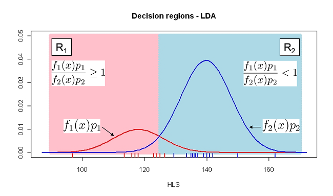
DAModel.2 <- lda(
  formula = Sex ~ HLS,
  data = Lizard,
  prior = c(0.8,0.2))
pred_mdl <- predict(DAModel.2)
confusion(Lizard$Sex, pred_mdl$class)
            True
Predicted     m          f
  m          13  2.0000000
  f           0 10.0000000
  Total      13 12.0000000
  Correct    13 10.0000000
  Proportion  1  0.8333333
N correct/N total = 23/25 = 0.92
In R the default choice of prior is “empirical” which means that the priors are set equal to the group proportions in the data set
Hence, if there are \(n_i\) observations in group \(i\) and \(N = \sum_{i=1}^g n_i\) is the total observation number, then
\[\hat{p}_i = \frac{n_i}{N}\] This may be reasonable if one assumes that the sample sizes reflect population sizes.
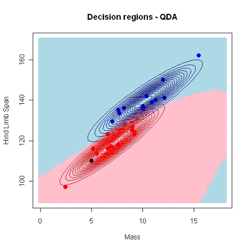
QDA differs from LDA in two ways:
library(MASS)
QDA_model <- qda(
  formula = Sex ~ HLS,
  data = Lizard,
  prior = c(0.8,0.2))
pred_mdl <- predict(QDA_model)
We often want to compare the performance of different classifiers.
Many available statistics for this purpose, but we will consider the accuracy or the apparent error rate (APER)
The performance of a classifier may as we’ve seen be summarized in a confusion matrix
From the error rate, we can also compute the classification accuracy
Consider the confusion matrix as,
| Male | Female | |
|---|---|---|
| Predicted | ||
| Male | \(n_m/m\) | \(n_m/f\) |
| Female | \(n_f/m\) | \(n_f/f\) |
| Total | \(n_m\) | \(n_f\) |
\[ \text{APER} = \frac{n_m/f + n_f/m}{n_m + n_f} = \frac{\text{Total Incorrect}}{\text{Total Observation}} \]
Classification accuracy will be \(1 - \text{APER}\).
DAModel.4 <- lda(
  formula = Sex ~ SVL,
  data = Lizard,
  prior = rep(0.5, 2))
pred_mdl <- predict(DAModel.4)
confusion(Lizard$Sex, pred_mdl$class)
            True
Predicted         m      f
  m          10.000  2.000
  f           3.000 10.000
  Total      13.000 12.000
  Correct    10.000 10.000
  Proportion  0.769  0.833
\[ \begin{aligned} P(\texttt{female | male}) &= \dfrac{3}{13} = 0.231 \\ P(\texttt{male | female}) &= \dfrac{2}{12} = 0.167 \end{aligned} \]
\[ \text{Apparent error rate (APER)} = \frac{3 + 2}{25} = 0.2 \]
Accuracy = \(1-\text{APER} = 0.8\)
As for regression models the errors based on fitted values may reflect over-fitting
Should have new test data to predict to get an honest classification error.
Alternatively we can perform cross-validation
K-fold cross-validation and
Leave-one-out (LOO) Cross-validation
da_model <- lda(
  formula = Sex ~ SVL,
  data = Lizard,
  prior = rep(0.5,2),
  CV = TRUE)

confusion(Lizard$Sex, da_model$class)
            True
Predicted         m     f
  m          10.000  3.00
  f           3.000  9.00
  Total      13.000 12.00
  Correct    10.000  9.00
  Proportion  0.769  0.75
Typically, as seen here, the accuracy goes down, and the APER increases when new samples are classified.
N incorrect/N total = 6/25 = 0.24
N correct/N total = 19/25 = 0.76