simrel-m
A simulation tool and its application
Supervisors:
11 June, 2017
Why simrel-m
-
By changing few parameters, we can simulate wide range of linear model data. For example,
- Controlling degree of multicollinearity in the simulated data
- Specifying the relevant principle components for prediction
- It is easy to use and has wide application

The idea behind

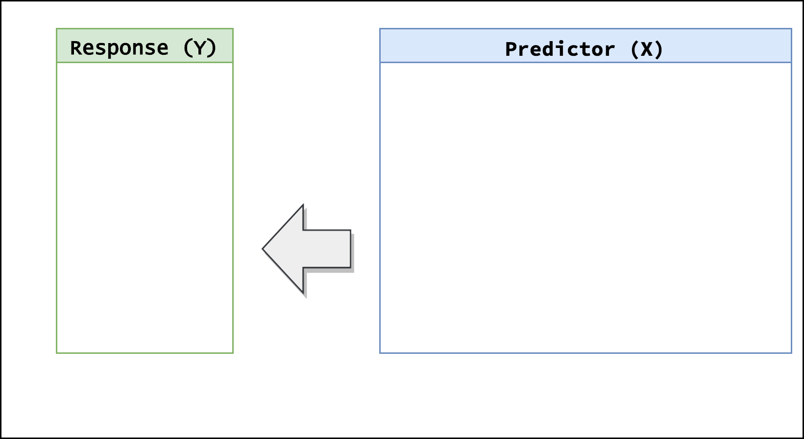
simrel[1] package
How it works


- Gets parameter setting from users
- Creates Covariance matrix
- Creates Rotation Matrix
- Rotates the sampled Latent variables
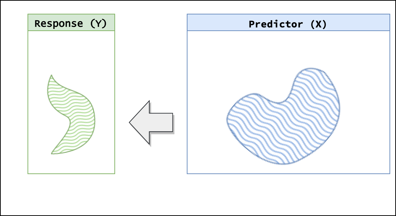
How it works


- Gets parameter setting from users
- Creates Covariance matrix
- Creates Rotation Matrix
- Rotates the sampled Latent variables
A Comparison
